

Introduction
EMI/EMC regulations are in place throughout the world to provide a level of protection and safety for users of electrical and electronic equipment. A great deal of time and effort goes into the design of today’s products to minimize their EMI signatures.
Many companies employ the services of a specialized test facility to perform the actual compliance tests required for EMI/EMC certification. The test facility might belong to an outside company (a “test house”) or to an in-house EMC department. Most engineers employ good design practices to minimize the potential for EMI/EMC problems. Even with the availability of accurate EMI/EMC simulation packages it is common today to perform “pre-compliance” measurements during the design and prototyping stages to identify and address potential EMI/EMC issues before the product is sent out for compliance testing. These techniques reduce the risk that the product will fail the final full compliance at the test house.
But What if the Product Fails Compliance Testing?
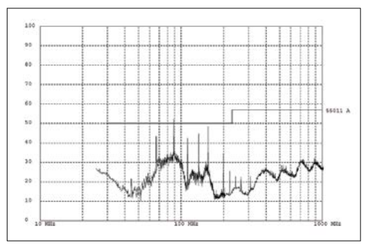
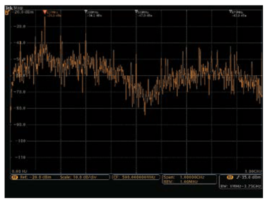
Even after employing good design, selecting high quality components, and taking time to carefully characterize the product, one can still be caught with an EMI issue! (Figure 1.)
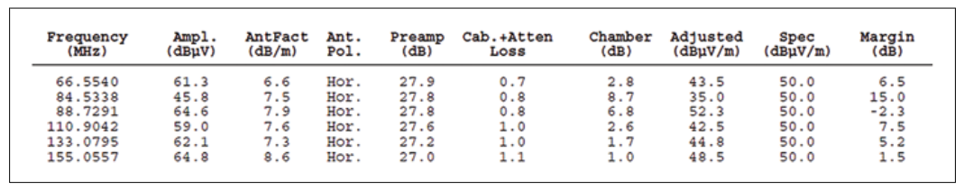
The above report indicates that there is a single peak which is above the limit for this specific standard. Normally in the report we will also receive the information in tabular format (Figure 2).
Understanding the EMI Report
At first glance EMI reports like the one above appear to provide straightforward information about a failure at a specific frequency. It should be a simple matter to identify which component of a design contains that source frequency and apply some attenuation in order to pass the test. Before sifting through the design to try and determine the source of the problem, one must understand how the test house produced this report.
The report in Figure 2 shows the test frequency, measured amplitude, calibrated correction factors, and adjusted field strength. The adjusted field strength is compared to the specification to determine the margin, or excess. While many of the test conditions are explicit in the report, some important things to think about may not be so apparent.
Frequency Range and Number of Test Points:
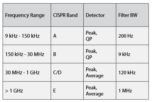
It is very unlikely that the frequency given in the test report is exactly the frequency of the EMI source. Frequency range and number of test points help determine how close the compliance test frequency is likely to be to the actual frequency of a source. According to the Special International Committee on Radio Interference (CISPR), when performing radiated emissions testing, different test methods must be used depending on frequency range. Each range requires a specific resolution bandwidth filter and detector type, as shown in Table 1. Frequency range determines the filter bandwidth and therefore the ability to resolve the exact frequency of interest.
Detector Type: In general the test house will first complete a peak scan as this test takes the least amount of time to complete. Quasi-peak (QP) scans take much more time to complete due to the nature of the detector (see sidebar, “Common Types of Peak Detection”). Quasi-peak detection uses a measurement weighting which places more emphasis on signals which could be interpreted as more “annoying” from a broadcast perspective, so it is possible that the detector type will mask the absolute amplitude of the offending signal.
Azimuth/Distance: When performing the scans the unit under test (UUT) may be placed on a turn-table so that information can be collected from multiple angles. This azimuth information is quite useful as it will indicate from which area of the UUT that the problem is emanating.
To further complicate matters the EMI/EMC test house will make their measurements in a calibrated RF chamber and report the results as a measure of field strength.
Fortunately, you do not need to duplicate test house conditions to troubleshoot EMI test failures. Instead of absolute measurements that are performed in the highly controlled EMI test facility, troubleshooting may be performed using the information in the test report, a good understanding of the measurement techniques used to generate the report, and relative observations taken around the UUT to isolate sources and gauge the effectiveness of remediation.
Common Types of Peak Detection
EMI measurements can be made with simple peak detectors. But the EMI department or the external test house use quasi-peak (QP) detectors. So you may wonder if you need a QP detector too.
The EMI department or the external labs typically begin their testing by performing a scan using simple peak detectors to find problem areas that exceed or are close to the specified limits. For signals that approach or exceed the limits, they perform QP measurements. The QP detector is a special detection method defined by EMI measurement standards. The QP detector serves to detect the weighted peak value (quasi-peak) of the envelope of a signal. It weights signals depending upon their duration and repetition rate. Signals that occur more frequently will result in a higher QP measurement than infrequent impulses.
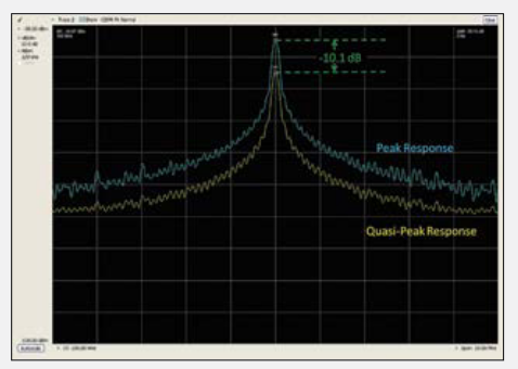
An example of peak and QP detection is seen in Figure 3. Here, a signal with an 8 μs pulse width and 10 ms repetition rate is seen in both peak and QP detection. The resultant QP value is 10.1 dB lower than the peak value.
A good rule to remember is QP will always be less than or equal to peak detect, never larger. So you can use peak detection to do your EMI troubleshooting and diagnostics. You don’t need to be accurate to an EMI department or lab scan, since it is all relative. If your lab report shows the design was 3 dB over and your peak detect is 6 dB over, then you need to implement fixes that reduce the signal by 3 dB or more.
Where Do I Start?
When we look at any product from an EMI perspective the whole design can be considered a collection of energy sources and antennas. To identify the source of an EMI problem we have to first determine the source of energy and second find out how this energy is being radiated. Common sources of EMI problems* include:
- Power Supply Filters
- Ground Impedance
- Inadequate Signal Returns
- LCD Emissions
- Component Parasitics
- Poor Cable Shielding
- Switching Power Supplies (DC/DC Converters)
- Internal Coupling Issues
- ESD In Metalized Enclosures
- Discontinuous Return Paths
* W. D. Kimmel, D. D. Gerke; “Ten Common EMI Problems in Medical Electronics”; Medical Electronics Design; October 1, 2005
While this list outlines some common sources of EMI it is by no means a definitive list. To determine the source of energy on a particular board engineers will often employ near field probes. When using these types of probes we must keep in mind the fundamentals of signal propagation.
To identify the particular source and antenna at the heart of a particular EMI problem, we can examine the periodicity and coincidence of observed signals.
Periodicity:
- What is the RF frequency of the signal?
- Is it pulsed or continuous?
These signal characteristics can be monitored with a basic spectrum analyzer.
Coincidence:
- What signal on the UUT coincides with the EMI event?
It is common practice to use an oscilloscope to probe the electrical signals on the UUT.
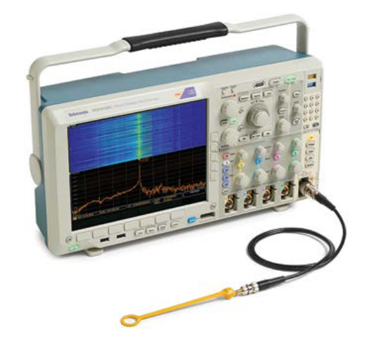
Examining the coincidence of EMI problems with electrical events is arguably the most time consuming process in EMI diagnostics. In the past it has been very difficult to correlate information from spectrum analyzers and oscilloscopes in a meaningful way. The introduction of the MDO4000 Series Mixed Domain Oscilloscope (see sidebar: “Mixed Domain Oscilloscopes”) has eliminated the difficulty of synchronizing multiple instruments for EMI troubleshooting.
Near Field vs. Far Field Measurements
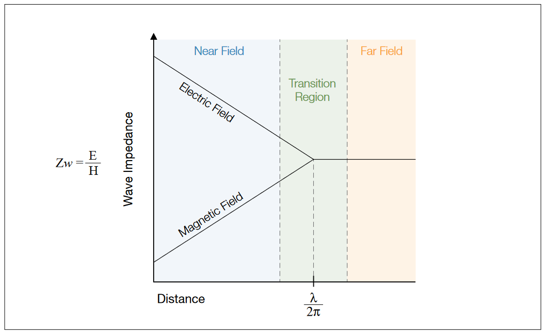
Figure 4 shows the behavior of wave impedance in the near and far fields, and the transition zone between them. We can see that in the near field region fields can range from predominantly magnetic to predominantly electric. Near field measurements are used for troubleshooting, since they allow one to pinpoint sources of energy and they may be performed without the need for a special test site.
However, compliance testing is performed in the far field and predicting far field energy levels from near field measurements can be complicated because the strength of the far field signal is dependent not only on the strength of the source, but also the radiating mechanism as well as any shielding or filtering that may be in place. As a rule of thumb, we must remember that we if are able to observe a signal in the far field then we should be able to see the same signal in the near field. However, it is possible to observe a signal in the near field and not see the same in the far field.
Near Field Probing
While compliance testing procedures are designed to produce absolute, calibrated measurements, troubleshooting can be performed in large part using relative measurements.
Near field probes are essentially antennas which are designed to pick-up the magnetic (H Field) or electric (E Field) variations. In general near field probes do not come with calibration data so they are intended for making relative measurements.
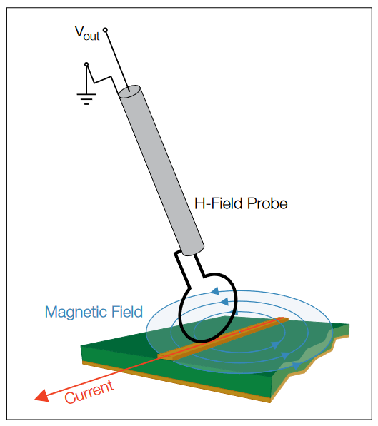
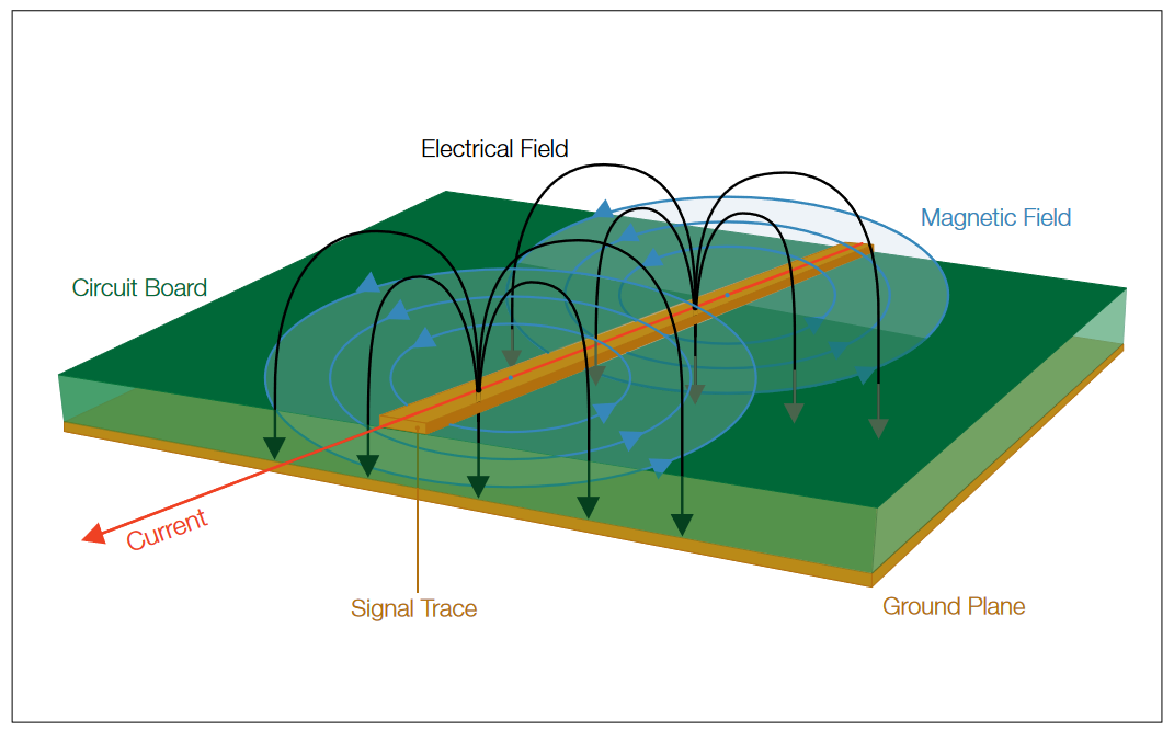
H-Field Probes
H-field probes have a distinctive loop design and should be held with the plane of the loop in-line with the current flow, such that the loop intersects the magnetic field lines of flux. The size of the loop determines the sensitivity, as well as the area of measurement, so care must be taken when using these types of probes to isolate a source of energy. Near field probe kits will often include a number of different sizes so that you can use a progressively smaller loop size in order to narrow the area of measurement. H-field probes are very good at identifying sources will relatively high current such as:
- low-impedance nodes & circuits
- transmission lines
- power supplies
- terminated wires & cables
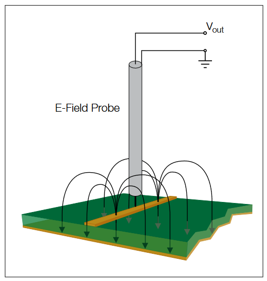
E-Field Probe
E-Field probes function as small monopole antennas, and respond to the electric field, or voltage changes. When using these types of probes it is important to keep the probe perpendicular to the plane of measurement. In practice E-field probes are ideally suited for zeroing in on a very small area, identifying sources with relatively high voltages as well as sources with no termination such as:
- high-impedance nodes & circuits
- unterminated PCB traces
- cables
At low frequencies, the circuit node impedances in a system can vary greatly, thus knowledge of the circuit or experimentation is required to determine whether an H-Field or E-Field probe will provide the most sensitivity. At higher frequencies, these differences are dramatic. In all cases, making repetitive relative measurements is important so that you can be confident that the near-field emission results from any changes implemented are accurately represented. The most important consideration is to be consistent in the placement and orientation of the near field probes for each experimental change.
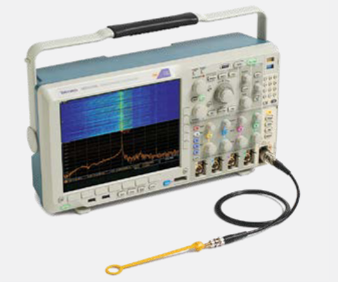
A mixed domain oscilloscope combines the measurement capabilities of an oscilloscope, spectrum analyzer and logic analyzer. The MDO4000 Series offers a unique ability to view analog signal characteristics, digital timing, bus transactions, and frequency spectra synchronized together. The MDO3000 also combines oscilloscope, spectrum analyzer, and logic analyzer capabilities, but it is not possible to acquire or view a frequency spectrum and time domain waveforms at the same time.
Case Study: Determining Signal Characteristics and Coincidence to Determine a Source
This case study will illustrate the process of gathering evidence to isolate an EMI source. An EMI scan of a small microcontroller indicated an over-limit failure from what appears to be a broadbanded signal centered around 144 MHz.
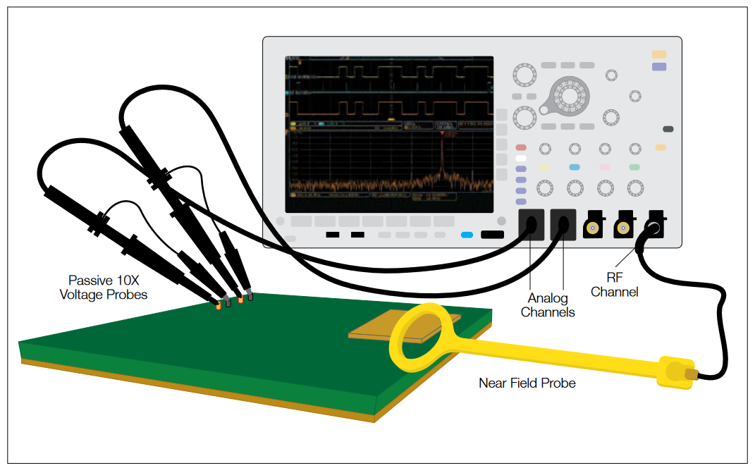
Using the spectrum analyzer of the MDO4000 (Figure 10) we first connect an H-field probe to the RF input so that we can localize the source of the energy.
It’s important to orientate the H-field probe so that the plane of the loop is in-line with the conductor being evaluated, thus positioning the loop so that magnetic field lines of flux pass through it. Moving the H-Field prove around the PCB, we can localize the source of energy. By selecting a narrower aperture probe we can focus the search in a smaller area.
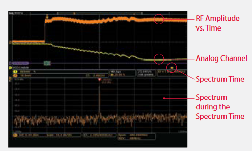
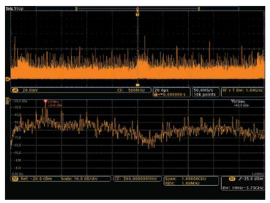
Once we have located the apparent source of energy, we turn on the RF Amplitude vs. Time trace (Figure 12). This trace shows the integrated power versus time for all signals in the span. We can clearly see a large pulse in display. Moving spectrum time through the record length we can see that the EMI event (wide band signal centered around 140 MHz) directly corresponds to the large pulse. To stabilize the measurement we can enable the RF power trigger and then increase the record length so that we can determine how often the RF pulse is occurring. To measure the pulse repetition period we could enable the measurement markers and directly determine the period.
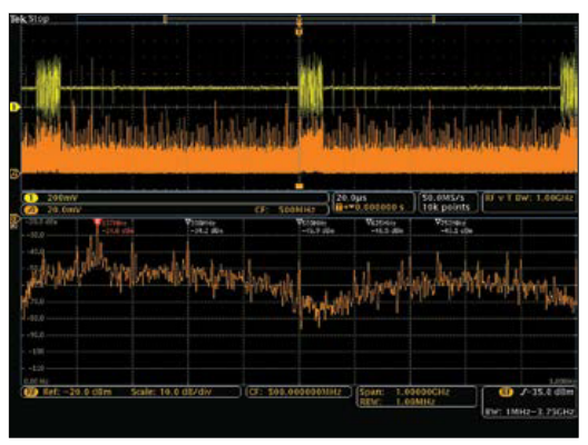
The next step to positively identify the source of EMI is to utilize the oscilloscope portion of the MDO4000 Series oscilloscope.Keeping the same setup we can now enable Channel 1 of the oscilloscope and browse the PCB looking for a signal source which is coincident with the EMI event.
After browsing signals with the oscilloscope probe for a while, the signal in Figure 13 was spotted. It can be clearly seen on display that the signal we are connected to on Channel 1 of the scope can be directly correlated to the EMI event.
Conclusion
Failing an EMI compliance test can put a product development schedule at risk. However, the troubleshooting techniques outlined here can help you isolate the source of the energy so you can formulate a plan for remediation. Effective troubleshooting requires understanding the compliance test report and how compliance testing and troubleshooting employ different measurement techniques. In general, it depends on looking for relatively high electromagnetic field, determining their characteristics, and correlating field activity with circuit activity to determine the source.