


Introduction
Clocks are the heartbeats of embedded systems, providing timing references and synchronization between components, subsystems,and entire systems. Incorrect clock signal amplitudes and timing can prevent reliable digital circuit operation. Noise and timing aberrations on clock signals can cause degraded or intermittent system performance, so thorough characterization of clock signals is a critical step in assuring reliable embedded system design.
This application note provides several examples of amplitude and timing measurements on digital clock signals,including
- Amplitude Measurements
- Frequency Stability Measurements
- Basic Jitter Analysis
- Overview of Advanced Jitter Analysis
This document uses the 5 Series MSO mixed signal oscilloscope to illustrate the measurements. The 6 Series MSO operates identically, but is available with higher bandwidth and offers lower input noise. Many of the measurements shown can be performed with other oscilloscopes, although the specific setups will vary. Some of the measurements in this application note take advantage of the optional Advanced Jitter Analysis application for the 5 and 6 Series MSOs.
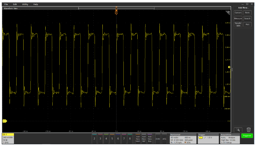
This display shows a 40 MHz clock signal captured with 12-bit vertical resolution on a 1 GHz bandwidth 5 Series MSO. To assure adequate signal fidelity, a 1 GHz differential probe was attached to the test points near the clock driver. Since the bandwidth of the measurement system is about 25 times the clock frequency, measurement errors due to bandwidth are minimal.
The oscilloscope’s fine vertical scale was adjusted so the signal fills most of the graticule (without going off the top or bottom) to optimize the vertical resolution.and a high real-time sample rate is selected to optimize timing resolution.
Amplitude Measurements
By visual inspection of the signal relative to the horizontal and vertical labels inside the graticule, you can determine that the clock’s low level is about 750 mV and the high level is about 2.4 V. The clock period is about 25 ns, which corresponds to 40 MHz. For some quick debug tasks, this measurement precision may be sufficient.
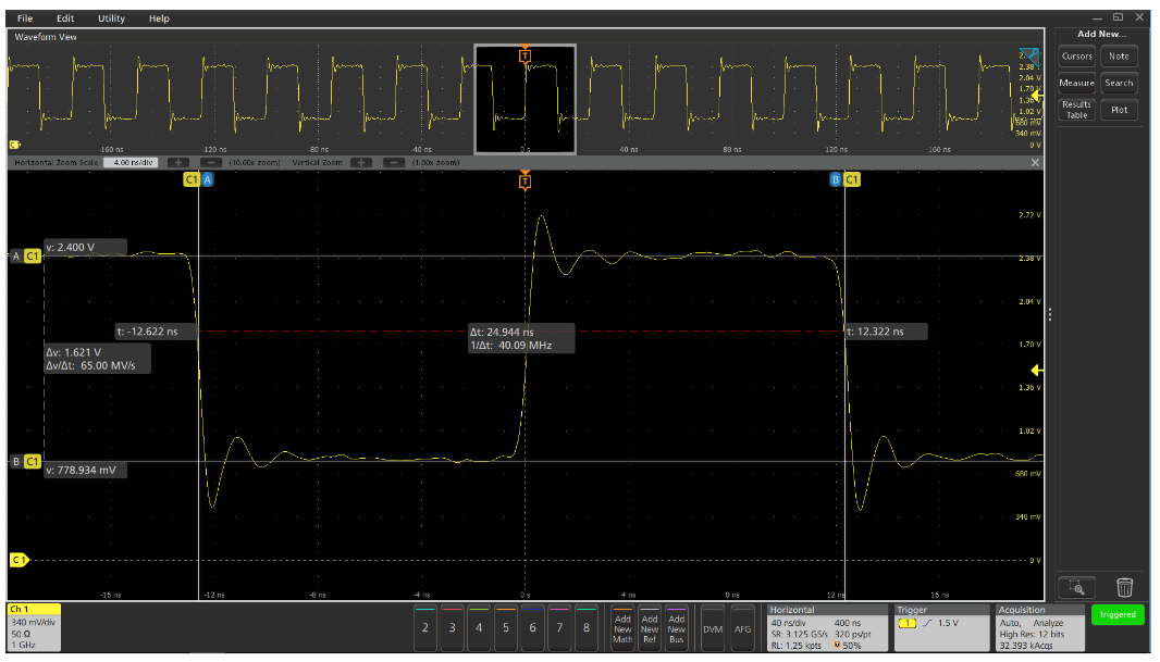
More precise amplitude and timing measurements can be made by zooming in on one cycle of the signal and using cursors. As you can see in the display above, the measurement resolution is significantly improved, but the measurements are based on a single cycle of the waveform and can be difficult to make if the signal is varying over time.
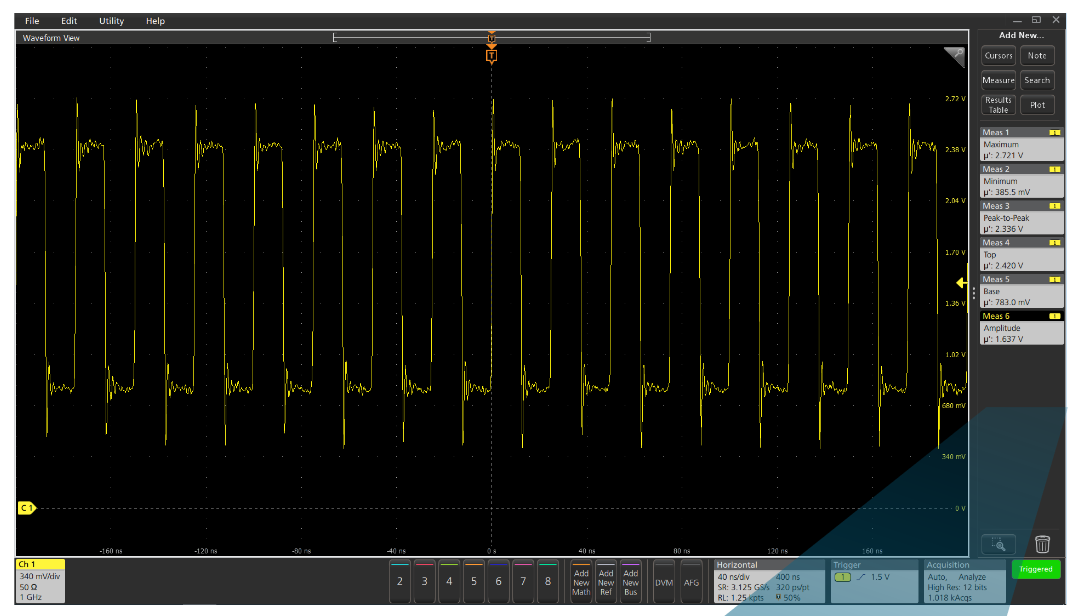
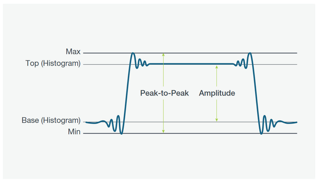
The automated measurement algorithms use digital signal processing on the digitized waveforms. Notice that the Top and Base measurements are similar to the ones previously made with the horizontal bar cursors, but with higher resolution.
Notice that the Peak-to-Peak measurement is equal to the difference between the Maximum and Minimum measurements, and the Amplitude measurement is equal to the difference between the Top and Base measurements.
These readings provide a good snapshot, but how are the measurement values varying over time?
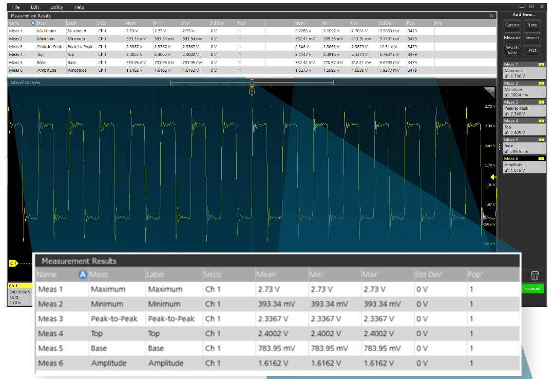
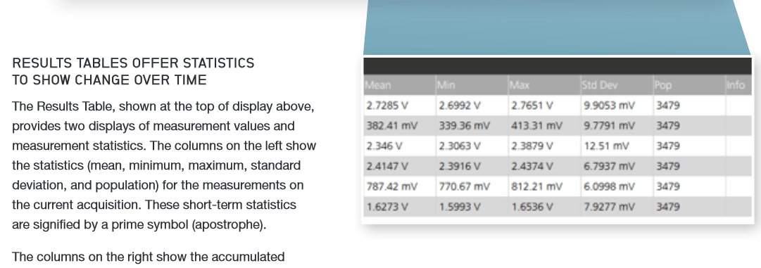
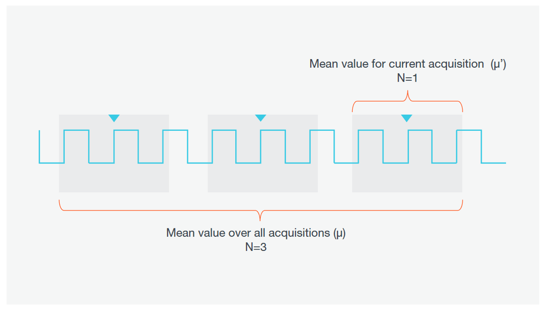
Measurement statistics over all acquisitions are calculated from the time the first acquisition is started through the current acquisition. This is useful for gaining insight into stability over longer time periods.
Based on the accumulated statistics of the amplitude measurements, you can compare the measurement values to the data sheets of the clock driver and the components being driven by the clock signal to verify that the amplitude characteristics are within the specifications. For example:
- The Max value of the Maximum measurement and the Min value of the Minimum measurement are within the receiver's absolute input voltage range spec.
- The Min value of the Top measurement is greater than the driver's VOHmin and the receiver's VIHmin spec.
- The Max value of the Base measurement is less than the driver's VOLmax and the receiver's VILmax spec.
Frequency Stability Measurements
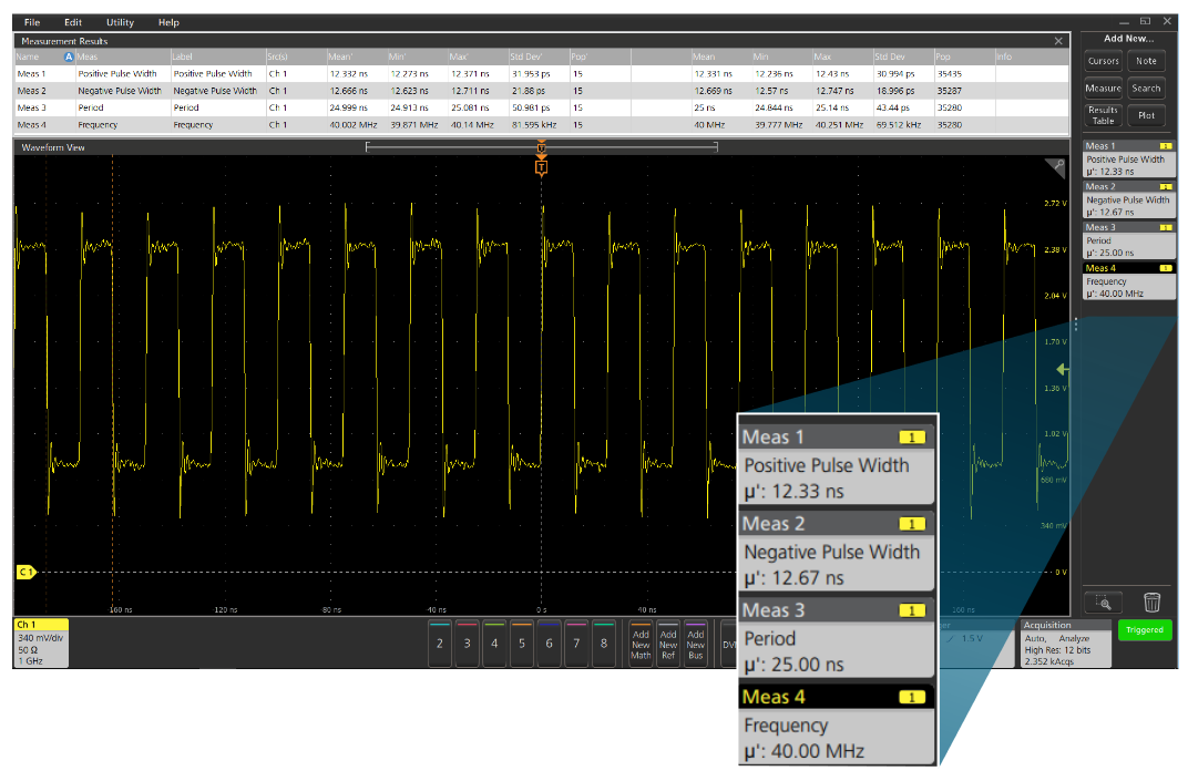
Similarly, automatic timing measurements can be used to provide quick horizontal measurements.The µ’ values shown in the measurement results badges at the right side of the display represent the mean timing measurement values for the current acquisition.
Notice that the Period measurement provides similar results to the measurement made with the V Bars cursors earlier in this application note, but with higher resolution and updating much more rapidly.
As expected, the Period measurement is equal to the sum of the Positive Pulse Width and Negative Pulse Width measurements, and the Frequency measurement is the reciprocal of the Period measurement.
From here, you can compare the measurements to the component data sheets of the receiver components that are driven by the clock signal to verify that the timing characteristics are within the specifications. For example:
- Max and Min values of the Frequency measurement are within the specified clock frequency (fclock) range.
- The Min value of the Positive Pulse Width measurement is greater than the minimum pulse duration spec tw (CLK high).
- The Min value of the Negative Pulse Width measurement is greater than the minimum pulse duration spec tw (CLK low).
Standard automated timing measurements provide a good starting point for jitter analysis, by verifying that the clock frequency is meeting specifications.Adding measurement statistics, such as minimum and maximum frequency,provides confidence that the clock pulses are continuous. And standard deviation (σ) provides a quantitative measure of the frequency stability over time. However, these statistics give little insight into the manner of frequency variation.
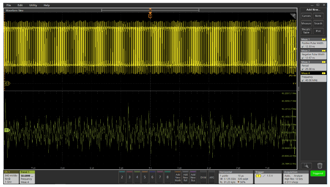
TIME TRENDS SHOW FREQUENCY VARIATION
In the screen above the acquisition time window has been increased to 10 µs to increase the number of cycles in the acquisition and thus the number of available cycle measurements.The time-correlated Time Trend display in the lower half of shows the variation of frequency measurements across the acquisition. This time trend display provides a better understanding of the frequency variation than the measurement statistics, but it is still difficult to determine if the variations are random or caused by systematic factors such as other nearby signals.
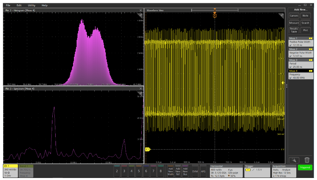
HISTOGRAMS AND SPECTRUM PLOTS PROVIDE MORE CLUES
The histogram of the frequency measurement values, in the upper left corner, suggests that the variations in the frequency are not completely random (not a classic Gaussian or bell curve).The shape would suggest that there may be other signals cross-talking into the clock signal.
The spectrum plot shows significant frequency components at about 7 MHz and 20 MHz.These measurements and knowledge of the rest of the design may be helpful in determining the root cause of the clock frequency variations, but it is difficult to know which of several potential causes is dominant. For that, we need to decompose the timing jitter into its components.
JITTER ANALYSIS TOOLS
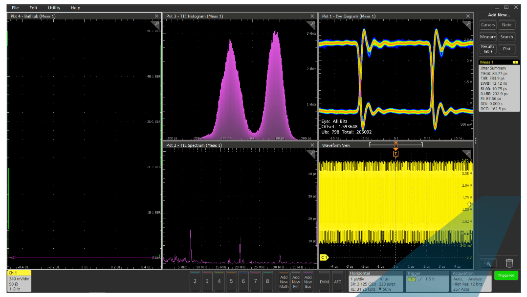
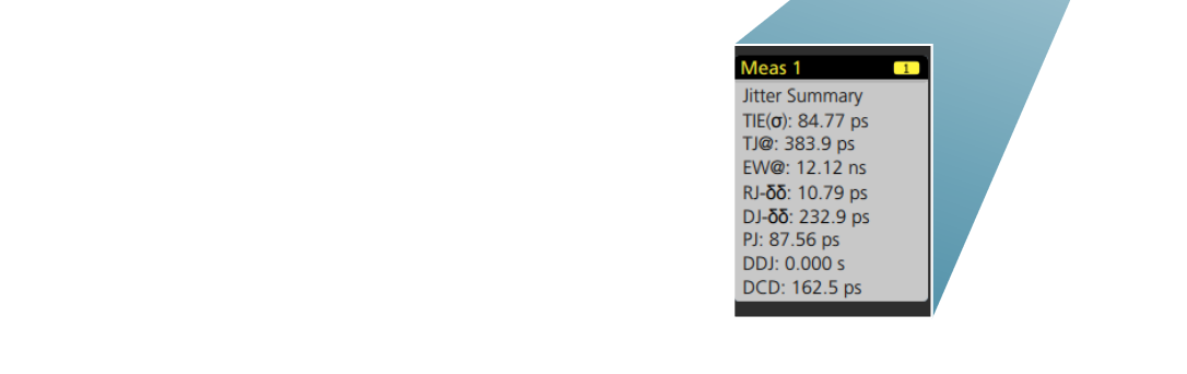
The base 5 Series measurement system includes Time Interval Error (TIE) and phase noise measurements. TIE quantifies the time variation of a clock signal from an ideal signal. An optional Advanced Jitter Analysis application provides a one-button analysis of the 40 MHz clock signal, shown above, including TIE analysis and an eye diagram. The measurement results badge at the right side of the screen above shows the automated measurement of Time Interval Error (TIE), a measure of timing relative to an ideal signal. Other measurements show the decomposition of the timing jitter into Total Jitter (TJ), Random Jitter (RJ),Deterministic Jitter (DJ), Periodic Jitter (PJ), Data-Dependent Jitter (DDJ),and Duty Cycle Distortion (DCD).
As predicted from the histogram of the frequency measurements, there is a systematic distortion of the clock. The deterministic jitter is much higher than random jitter, and the deterministic jitter is dominated by duty cycle distortion. The spectrum display in the bottom center of the screen above shows significant jitter components at 7.1 MHz, 20 MHz, and 30.3 MHz. In this case, a nearby 7.1 MHz clock proved to be the aggressor, interfering with the 40 MHz clock signal.
USING INFINITE PERSISTENCE TO FIND INTERMITTENT FAILURES
While examining the same circuit on a different prototype board, we noticed an occasional circuit malfunction. However, there wasn't any obvious problem when viewing the clock signal on the display.
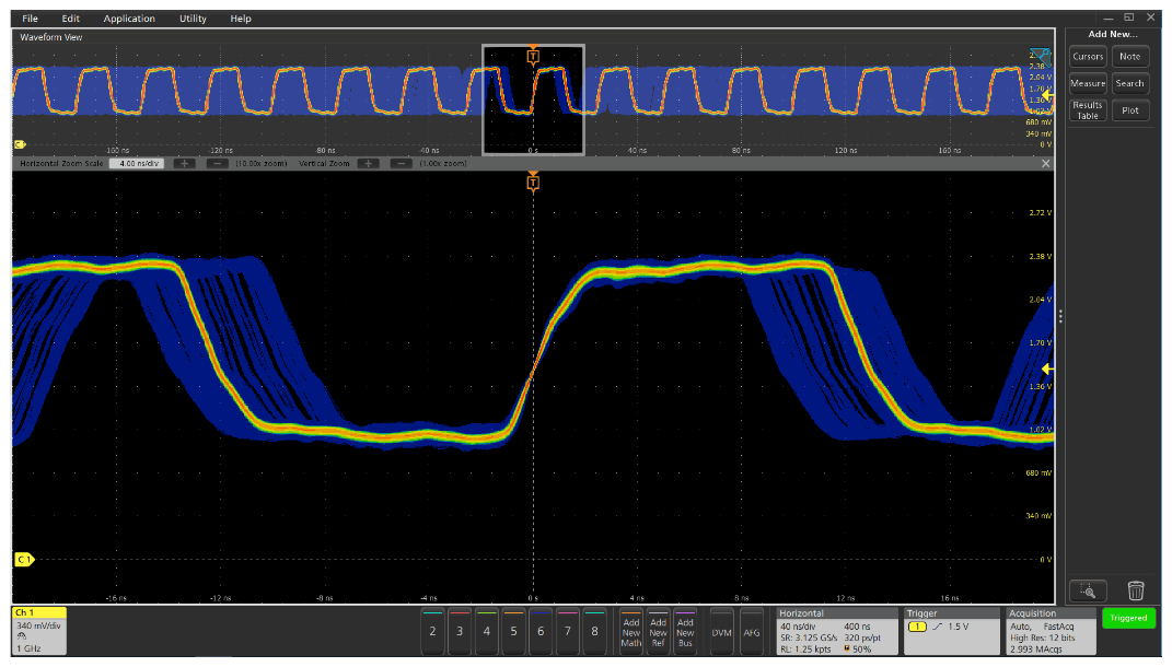
The 5 Series MSO offers an acquisition mode to quickly capture millions of the 40 MHz clock signals and overlay them on the display. This is called FastAcq mode and once it is activated we can quickly see that there are some very significant frequency variations on the clock signal on this defective board.
The FastAcq display is "temperature-graded". The wide frequency variations are shown in blue color, indicating that they are relatively rare.
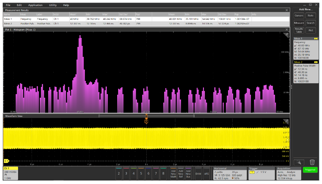
Now that we know these variations are there, we can plot the frequency measurements on a histogram with a logarithmic Y-axis to better understand the variations. (Using the logarithmic scale lets us see more detail at the low end of the scale.)
After allowing over 10 million frequency measurements to accumulate, the truly infrequent nature of the frequency variation appears. The average frequency is very accurate, but occasionally drifts as low as 35 MHz and as high as almost 55 MHz.
Without such statistical measurement techniques, infrequent anomalies such as these can easily go undetected.
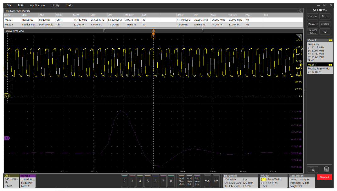
Now that we know that the frequency occasionally decreases, we can use pulse width triggering to capture abnormally wide pulses and capture the errors. In this example, the scope is set to trigger on a pulse width greater than 14 ns, which is more than the nominal 12.5 ns. The frequency trend at the bottom of the display shows graphically the frequency excursion above and below the 40 MHz ideal.
Further analysis of this clock circuit showed that the phase-locked loop controller was occasionally being reset. When this happened, the voltage-controlled oscillator circuit lost lock and momentarily shifted from the proper frequency.
Find more valuable resources at TEK.COM
Copyright © Tektronix. All rights reserved. Tektronix products are covered by U.S. and foreign patents, issu ed and pending. Information in this publication supersedes that in all previously published material. Specification and price change privileges reserved. TEKTRONIX and TEK are registered trademarks of Tektronix, Inc. All other trade names referenced are the service marks, trademarks or registered trademarks of their respective companies.
07/18 48W-61379-1